Logistic regression is a statistical method used for binary classification tasks. It is used for predicting the categorical dependent or target variable using a given set of independent variables or given features.

For Example,

The mouse is obese - YES or NO.

In the above example, the weight could be an independent feature to predict whether a mouse is obese or not this is a categorical dependent feature.

When you can use Logistic Regression:

• The dependent variable is categorical in nature.

• The independent variables in a regression model are not highly correlated with each other.

We are going to learn everything about logistic regression by applying on the Example Sit tight! And get ready for the most thrilling journey

Data Set

I will first tell you about the data set on which we are going to apply logistic regression to predict the target value

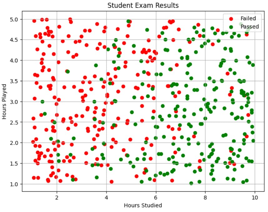
So our data set has three features, feature 1 is the number of hours student study feature 2 is the number of hours student plays and the third feature is whether they passed the exam or not.

We are going to train the model on Feature 1 and Feature 2 so that the model can learn to predict whether a student will pass or fail the exam.

# Set a random seed for reproducibility
np.random.seed(42)

# Number of samples in the dataset
num_samples = 500

# Generate random values for "Hours_Studied" between 1 and 10
hours_studied = np.random.uniform(1, 10, num_samples)

# Generate random values for "Hours_Played" between 1 and 5
hours_played = np.random.uniform(1, 5, num_samples)

# Define a function to simulate exam results based on "Hours_Studied" and "Hours_Played"
def simulate_passed_exam(hours_studied, hours_played):
    # We'll use a sigmoid function to simulate the probability of passing the exam
    probability_passed = 1 / (1 + np.exp(-(-3 + 0.8 * hours_studied - 0.5 * hours_played)))
    # Random binary values (0 or 1) based on the probability of passing
    return np.random.binomial(1, probability_passed)
# Generate the "Passed_Exam" values based on the "Hours_Studied" and "Hours_Played" values
passed_exam = simulate_passed_exam(hours_studied, hours_played)

# Create the dataset as a dictionary
dataset = {
    "Hours_Studied": hours_studied,
    "Hours_Played": hours_played,
    "Passed_Exam": passed_exam
}
# Convert the dataset dictionary to a pandas DataFrame
df = pd.DataFrame(dataset)
# Display the first few rows of the dataset
print(df.head())

Top five values of the Data:

This is how data looks like when we plot hours_played on the y-axis and hours_studied on the x-axis:

Sigmoid Function

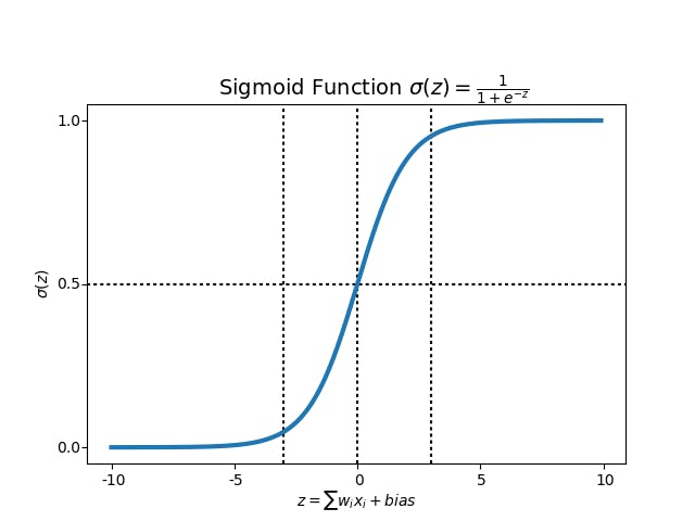
The sigmoid function is a mathematical function, which can transform any value between numbers 0 and 1. The sigmoid function 'squashes' the input values into the range [0, 1], making it suitable for converting real-valued predictions into probabilities.

The sigmoid function takes any real number as input and outputs a value between 0 and 1.

The mathematical formula of the sigmoid function is

def sigmoid(z): 
    # calculate the sigmoid of z
    h = 1/(1+(np.e)**(-z))
    return h

Now, what is this z in the function

Logistic regression takes a regular linear regression and applies a sigmoid to the output of the linear regression.

Regression:

We will refer to 'z' as the 'logits'.

The 𝜃 values are "weights". Some represent this 𝜃 as 'w' also. In this blog, we are going to use 𝜃 to refer to weight.

Ok, but what this weight is:

"weights" refer to the coefficients assigned to each feature in the model. These weights determine the strength and direction of the influence of each feature 'x' on the predicted outcome.

At the start of training, weights are assigned random values. As training progresses, the model updates these weights to minimize the loss function.

For the given dataset logits is:

z = bias + hours_studied 𝜃1 + hours_played * 𝜃2

This bias is another learnable parameter. It is an offset term that allows the model to make predictions even when all input features are zero.

Cost Function

The loss function measures the difference between the predicted value and the true value. The goal is to minimize this difference, indicating that the model's predictions align closely with the true values.

To achieve this, you use a different algorithm, such as the gradient descent algorithm, to update the weights and bias of the model. By doing so, you can minimize this loss function, which means you are trying to decrease the difference between the predicted value and the true value.

The loss function for a single training example is:

• All the ℎ values are between 0 and 1, so the logs will be negative. That is the reason for the factor of -1 applied to the sum of the two loss terms.

• When the true label y(i) is 1, the loss function will be: Loss = -log(ℎ(z(𝜃)(i))) In this case, we want the predicted probability ℎ(z(𝜃)(i)) to be close to 1, so the loss is minimized when the predicted probability is high.

• When the true label y(i) is 0, the loss function will be: Loss = -log(1 - ℎ(z(𝜃)(i))) In this case, we want the complementary probability (1 - ℎ(z(𝜃)(i))) to be close to 1, so the loss is minimized when the predicted probability for the negative class is high.

• When the true label y(i) is 1, but the predicted probability ℎ(z(𝜃)(i)) is close to 0, the loss will be very high. As ℎ(z(𝜃)(i)) approaches 0, log(ℎ(z(𝜃)(i))) approaches negative infinity, resulting in a large positive loss.

• When the true label y(i) is 0, but the predicted probability ℎ(z(𝜃)(i)) is close to 1, the loss will be very high. As ℎ(z(𝜃)(i)) approaches 1, log(1 - ℎ(z(𝜃)(i))) approaches negative infinity, resulting in a large positive loss.

The cost function used for logistic regression is the average of the log loss across all training examples:

• 𝑚 is the number of training examples

• 𝑦(𝑖) is the actual label of the training example 'i'.

• ℎ(𝑧(𝜃)𝑖) is the model's prediction for the training example 'i'.

Gradient Descent

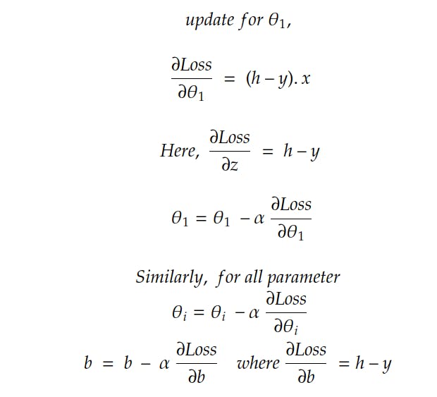
We use a gradient descent algorithm to minimize the loss or cost function. By updating the weight and bias we try to minimize the loss function. To learn more about the gradient descent algorithm click on this link.

The equation for the gradient descent:

• The learning rate 𝛼 is a value that we choose to control how big a single update will be.

• ∇𝜃𝑗 is the gradient (∂J(𝜃)/∂𝜃).

• 𝜃𝑗 is the value of the weight.

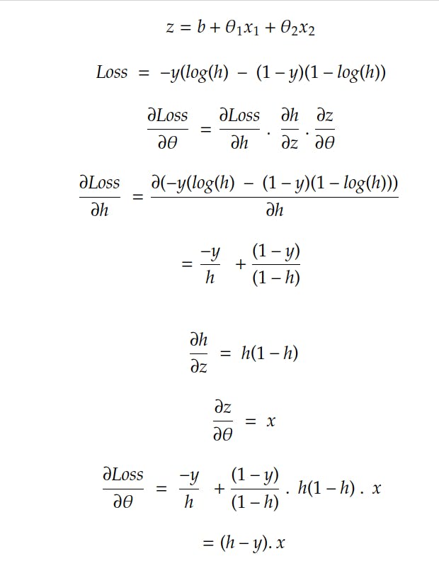
Now we will find ∂Loss / ∂𝜃 :

So when applying on the cost function

Code to find the gradient descent:

def gradientDescent(x, y, theta, alpha, num_iters):
    # get 'm', the number of rows in matrix x
    m = x.shape[0]

    for i in range(0, num_iters):

        # get z, the dot product of x and theta
        z = np.dot(x,theta)

        # get the sigmoid of z
        h = sigmoid(z)

        # calculate the cost function
        J = -1/m*(y.T @ np.log(h) + (1-y).T @ np.log(1-h))

        # update the weights theta
        theta =  theta - ((alpha/m)*(np.dot(x.T,h-y)))

    print(J)
    J = float(J)
    return J, theta

Training The Model

J, theta = gradientDescent(X_train, y_train, np.zeros((3, 1)), 0.01, 10000)
print(f"The cost after training is {J:.8f}.")
print(f"The resulting vector of weights is {[round(t, 8) for t in np.squeeze(theta)]}")

# output
[[0.46222476]]
The cost after training is 0.46222476.
The resulting vector of weights is [-1.93388363, 0.6061359, -0.47531684]

After training, we get the values of the weights as: [-1.93388363, 0.6061359, -0.47531684].

To predict whether a student will pass or fail, we multiply the weight values with the features, which gives us the value of z.

Next, we pass this z through a sigmoid function to obtain the probability. If the probability is greater than 0.5, it means the student will pass; otherwise, they will fail.

Note: We have divided the data in the train and test set in the ratio of 7:3.

Testing The Model

# Calculate the dot product of the test set and the learned weights
z_test = np.dot(X_test, theta)

# Get the sigmoid of the dot product to obtain predicted probabilities
predicted_probabilities = sigmoid(z_test)

# Threshold the probabilities to get binary predictions (0 or 1)
predicted_labels = (predicted_probabilities >= 0.5).astype(int)

# Compare predicted labels to actual labels (y_test)
accuracy = np.mean(predicted_labels == y_test)

print(f"Accuracy on the test set: {accuracy*100:.2f}%")

# output
Accuracy on the test set: 81.46%

Note: I didn't include the code blog for dividing the train and test sets. If you're interested in further exploration, data manipulation, or enhancing the model, you can find the link here of the notebook.