
Gradient descent is a common optimization approach in machine learning and numerical optimization. It is an iterative method to find the minimum (or maximum) of a function by changing the function's parameters or variables in the direction of the steepest descent (or ascent) of the function's gradient.
Note: To perform gradient descent on any function, the function should be continuous and differentiable at least within the domain of interest.
What is Gradient?
In the case of single-variable functions, the gradient corresponds to the first derivative of the function. The first derivative measures the slope of the function with respect to that single variable.
In the case of multi-variable functions, the gradient is a vector that comprises the partial derivatives of the function with respect to each variable. Each component of the gradient vector represents the rate of change or the slope of the function along the corresponding dimension or variable.
For a function f(x₁, x₂, ..., xn) with multiple variables, the gradient at a given point p is denoted as ∇f or grad(f) and is represented as a vector:
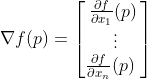
Here, ∂f/∂xi represents the partial derivative of the function f with respect to the variable xi.
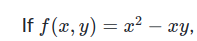
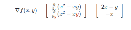
then,
Algorithm
Steps to find the local minima of the function:
Initialize the local minima with some random value.
Calculate the gradient of the function at the current local minimum.
Update the local minimum by subtracting the gradient multiplied by a learning rate.
Repeat steps 2 and 3 for a certain number of iterations or until a convergence criterion is met.
# Define the function f(x) and its derivative df(x)
def fx(x):
    return 3*x**2 +3  # function

def deriv(x):
    return 6*x  #  derivative of function

# random starting point
localmin = np.random.choice(x,1)   # here x is an array of some
                # random.choice(x,1) is choosing any single random number from the array x
# learning parameters
learning_rate = .01
training_epochs = 100    # this will repeat step 2 and 3 for the 100 times

# run through training
for i in range(training_epochs):
  grad = deriv(localmin)   # gradient is the derivative of the function at localmin point
  localmin = localmin - learning_rate*grad
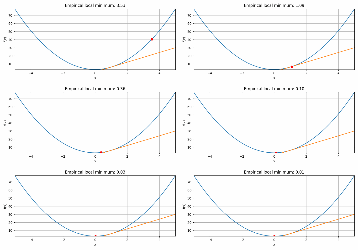
Showing how this algorithm works by solving it for three iterations:
Function f(x) = 3x^2 + 3
Derivative of f(x), df(x)/dx = 6x
Starting point (localmin) = 4
Learning rate (α) = 0.01
Number of iterations (training_epochs) = 3

Iteration 1:
let initial localmin = 4
f(4) = 3(4)^2 + 3 = 51
df(4)/dx = 6(4) = 24

Update rule:
localmin_new = localmin - α * df(localmin) = 4 - 0.01 * 24 = 3.76

Iteration 2:
At localmin = 3.76:
f(3.76) = 3(3.76)^2 + 3 ≈ 44.9856
df(3.76)/dx = 6(3.76) ≈ 22.56

Update rule:
localmin_new = localmin - α * df(localmin) = 3.76 - 0.01 * 22.56 ≈ 3.5344

Iteration 3:
At localmin = 3.5344:
f(3.5344) = 3(3.5344)^2 + 3 ≈ 40.4759
df(3.5344)/dx = 6(3.5344) ≈ 21.2064

Update rule:
localmin_new = localmin - α * df(localmin) = 3.5344 - 0.01 * 21.2064 ≈ 3.322336

After 3 iterations, the approximate updated localmin is 3.322336.
Learning Rate: It determines the step size or the speed at which the optimization algorithm moves towards the optimal solution.
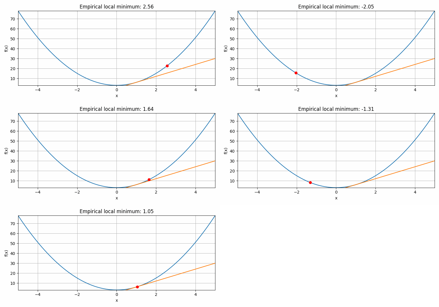
Choosing an appropriate learning rate is essential. If the learning rate is set too high, the algorithm may overshoot the optimal solution, resulting in instability and divergence. The point or parameters being optimized may oscillate or jump around, failing to converge. On the other hand, if the learning rate is set too low, the algorithm may converge very slowly, taking a long time to reach the optimal solution or getting stuck in a suboptimal solution.
Gradient: It provides information about the steepest ascent or descent direction at a specific point, which is useful in optimization algorithms like gradient descent to iteratively move towards the direction of the steepest descent and potentially converge to a local or global minimum of the function.
If the learning rate is set too high-
Applying gradient descent on a multivariable equation
Let the function is:
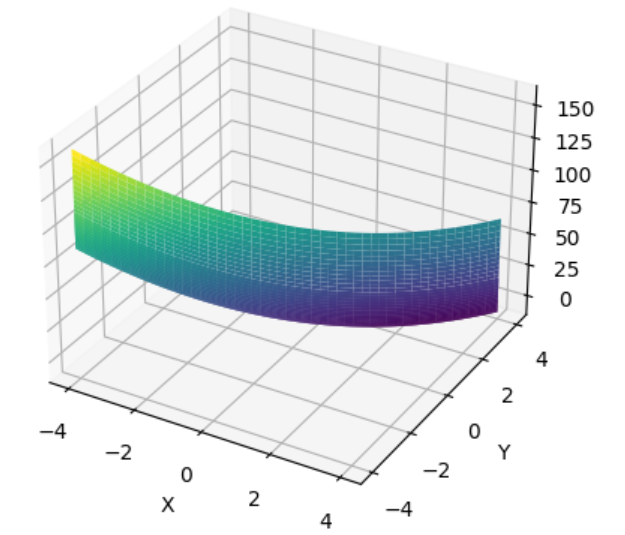
f(x, y) = 2x^2 + 3y^2 - 12x - 6y + 9
The partial derivatives of f(x, y) are:
∂f/∂x = 4x - 12
∂f/∂y = 6y - 6
This is how the function looks on the graph
And this is how the function looks like from the above
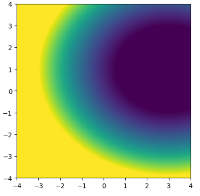
The above graph shows the top view of the function; the point where the value of f(x,y) is greater than 60 is represented by yellow, and the point where the value of f(x,y) is less than 0 is represented by dark blue, and the value between 0 and 60 is a mix of yellow and blue.
We can see from the graph that the graph has the darkest blue color at (3, 1), meaning this is the global minimum of the graph.
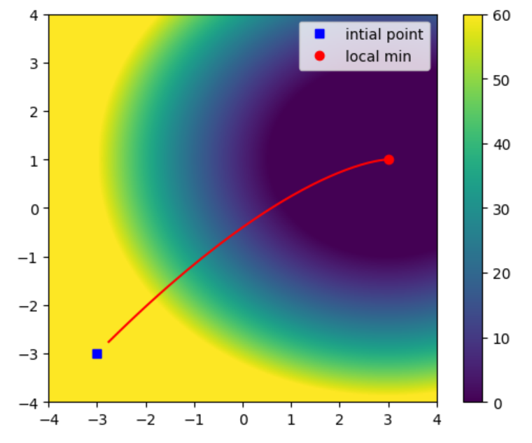
Now, we will find the minimum by applying the gradient descent algorithm-
# create derivative functions using sympy
x,y = sym.symbols('x,y')
Z =  2*x**2 + 3*y**2 - 12*x - 6*y + 9
# create functions from the sympy-computed derivatives
df_x = sym.lambdify( (x,y),sym.diff(Z,x),'sympy' )
df_y = sym.lambdify( (x,y),sym.diff(Z,y),'sympy' )

# starting point
localmin =  [-3,-3]
intialpoint = localmin[:] # make a copy

# learning parameters
learning_rate = .01
training_epochs = 1000

# run through training
trajectory = np.zeros((training_epochs,2))
for i in range(training_epochs):
  grad = np.array([ df_x(localmin[0],localmin[1]),
                    df_y(localmin[0],localmin[1])
                  ])
  localmin = localmin - learning_rate*grad  # add _ or [:] to change a variable in-place
  trajectory[i,:] = localmin


print(localmin)
print(intialpoint)
# output
[3. 1.]
[-3, -3]
Above we have used sympy library to compute the partial derivative of the function f(x,y).
Showing how this algorithm works by solving it for three iterations:
f(x, y) = 2x^2 + 3y^2 - 12x - 6y + 9
Starting point: (-3, -3)
Learning rate: 0.01

Iteration 1:
Compute the gradient:
∂f/∂x = 4x - 12
∂f/∂y = 6y - 6

Evaluate the gradient at the starting point:
df/dx = 4(-3) - 12 = -24
df/dy = 6(-3) - 6 = -24

Update the local minimum point:
x = x - learning_rate * df/dx = -3 - 0.01 * (-24) = -2.76
y = y - learning_rate * df/dy = -3 - 0.01 * (-24) = -2.76

Iteration 2:
Compute the gradient:
df/dx = 4x - 12
df/dy = 6y - 6

Evaluate the gradient at the updated point:
df/dx = 4(-2.76) - 12 = -23.04
df/dy = 6(-2.76) - 6 = -22.56

Update the local minimum point:
x = x - learning_rate * df/dx = -2.76 - 0.01 * (-23.04) = -2.5296
y = y - learning_rate * df/dy = -2.76 - 0.01 * (-22.56) = -2.5344

Iteration 3:
Compute the gradient:
df/dx = 4x - 12
df/dy = 6y - 6

Evaluate the gradient at the updated point:
df/dx = 4(-2.5296) - 12 = -22.1184
df/dy = 6(-2.5344) - 6 = -21.2064

Update the local minimum point:
x = x - learning_rate * df/dx = -2.5296- 0.01 * (-22.1184) = -2.308416
y = y - learning_rate * df/dy = -2.5344 - 0.01 * (-21.2064) = -2.322336

After 3 iterations, the updated local minimum point is approximately (-2.308, -2.322).
Potential Problems with gradient descent
Localmin
Gradient Descent is guaranteed to go downhill, but it doesn't guarantee finding the correct or best solution. There is a possibility that it gets stuck at the local min, which is the worst local minima among all the local minima.
Even after this problem, gradient descent works really well.
One reason for that could be that there are many good solutions (and many equally good local minima) present in a curve.
Another reason could be that gradient descent gets trapped in local minima only if that point is the minimum in all dimensions.
Solution of this problem:
Retrain the model many times using different random weights (different starting locations on the loss curve) and pick the model that works the best.
Increase the dimensionality (complexity) of the model to have fewer local minima.
Saddle Point
A saddle point is a critical point in a function where the first-order partial derivatives are equal to zero, but it is neither a local minimum nor a local maximum. In other words, it is a point on the function's surface where the curvature changes in different directions.
Geometrically, a saddle point resembles a saddle, where one direction is concave (curving downward) and the other direction is convex (curving upward).
Saddle points pose challenges for gradient-based algorithms such as gradient descent because the gradient becomes zero, leading to convergence issues.
Solution of this problem:
Random restarts: In some cases, saddle points can be local optima, and random restarts can help overcome them.
Momentum-based optimization: Momentum helps the optimization algorithm to continue moving even in the presence of saddle points.
Conclusion
Gradient descent is an iterative optimization algorithm used to find the minimum of a function. It relies on the concept of gradients, which indicate the direction of the steepest descent, to update the current estimate of the minimum. By iteratively adjusting the estimate in the direction of the negative gradient, gradient descent aims to converge to the optimal solution.
Overall, gradient descent is a powerful and versatile optimization algorithm that forms the foundation of many machine learning models and optimization techniques. Its effectiveness relies on careful parameter tuning and understanding the properties of the problem at hand.


